Nearpod version available
Using Systems of Equations with Supply and Demand Application
Objective
Students will be able to:
- Define supply, demand, law of demand, and equilibrium.
- Construct a supply and demand graph.
- Compute the equation of a linear demand curve.
- Compute the equation of a linear supply curve.
- Compute the intersection of the supply curve and demand curve (confirm the equilibrium price and quantity) using a system of equations.
Concepts

In this personal finance lesson, students will learn supply and demand by utilizing a system of equations.
Resources
- Activity 1 – Activity 4, one copy per student
- Graph paper, one sheet per student
- Episode 1: Supply from the Federal Reserve Bank of St. Louis’ Economic Low Down Video Series – Stop the video at 2:08.
- Episode 2: Demand from the Federal Reserve Bank of St. Louis’ Economic Low Down Video Series – Stop the video at 2:44.
- https://www.stlouisfed.org/education/economic-lowdown-video-series/episode-3-equilibrium from the Federal Reserve Bank of St. Louis’ Economic Low Down Video Series – Stop the video at 3:15.
Procedure
Supply and demand is the meat and potatoes of all economic analysis. In this lesson students will get an introduction by creating equations and graphing them to find the equilibrium points. They will have the opportunity to put their Algebra 1 math skills to work in a real world situation by mathematically determining the equilibrium price and quantity using a system of equations.
- Introduce the lesson by asking the following: how are prices determined? [Answers will vary. Guide students to the correct response that it is the interaction of consumers and producers: the interaction of supply and demand.]
- Introduce and define demand. [Demand is the quantity of a good or service that buyers are willing and able to buy at all possible prices during a period of time.]
- Introduce and define the law of demand. [The law of demand states that as the price of a good or service rises (or falls), the quantity of that good or service that people are willing and able to buy during a certain period of time falls (or rises).]
- Distribute a copy of Activity 1 to each student. Give students a moment to review the questions. Explain that they will fill in the blanks as they watch a couple of short video clips.
- Reinforce these concepts by showing Episode 2: Demand from the Federal Reserve Bank of St. Louis’ Economic Lowdown Video Series: Episode 2: Demand. (Only show video through 2:44. The remainder of the video is beyond the scope of this introductory lesson).
- Review the answers to the demand portion of Activity 1 using Activity 1 Answer Key.
- Introduce and define supply. [Supply is the amount of a good or service that producers are willing and able to offer for sale at each possible price during a given period of time.]
- Explain that typically, as the price of a good or service rises (or falls), the quantity of that good or service producers are willing to produce and sell increases (or decreases).
- Reinforce these concepts by showing Episode 1: Supply from the Federal Reserve Bank of St. Louis’ Economic Low Down Video Series: Episode 1: Supply (Only show video through 2:08. The remainder of the video is beyond the scope of this introductory lesson).
- Review the answers to the supply portion of Activity 1 using the Activity 1 Answer Key.
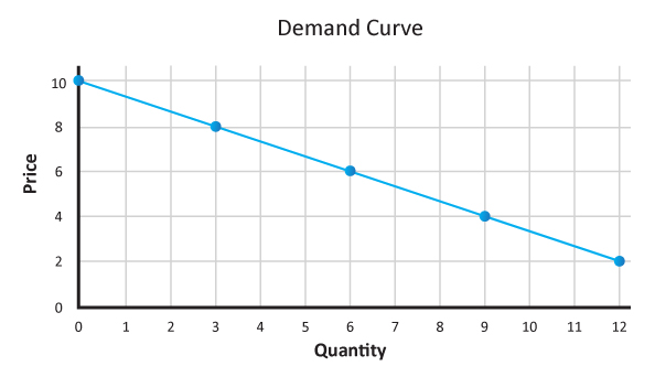
- Demonstrate the law of demand, explaining that each student has $10 to spend on brownies. Draw a chart like the one below on the board. Ask the students: “How many brownies are you willing and able to buy at each of the following prices?” Create your own demand schedule based on the number of brownies students are willing and able to buy at each price (Note: it is acceptable if the demand schedule is not linear for this section of the lesson, but is better if consistent).
| Price (y axis) | Quantity Demanded (x axis) |
|---|---|
| Price (y axis) | Quantity Demanded (x axis) |
| $10 | 0 |
| $8 | 3 |
| $6 | 6 |
| $4 | 9 |
| $2 | 12 |
- Ask what the relationship is between prices and quantities demanded. [Indirect or inverse relationship – as the price increases, the quantity demanded decreases and, vice versa, as the price decreases, the quantity demanded increases.] Remind students that this indirect relationship is known as the law of demand.
- Distribute a sheet of graph paper to each student. Have students follow along and graph the demand curve as you draw the curve on the board.
- Draw a demand curve as a downward sloping line using the data provided by the students. Reiterate the indirect relationship between the two variables – price and quantity demanded.
As an example, here is a graph of provided data.

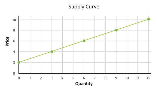
- Explain supply by telling students that you are a brownie producer/supplier and that you are willing and able to supply the following amounts of brownies at each price. Note to teacher: because you want the demand and supply graphs to intersect, base your supply schedule on the class demand schedule. See example below:
Supply Schedule Price (y axis) Quantity Supplied
(x axis)$10 12 $8 9 $6 6 $4 3 $2 0 - Ask how we describe a relationship like the one we see between the price and quantity supplied. [Direct or positive relationship – as the price increases, the quantity supplied increases and, vice versa, as the price decreases the quantity supplied decreases.] Explain this is consistent with the concept introduced in item #8 above.
- Ask students to plot the data from the supply schedule and draw a graph on their graph paper.
- Draw a supply curve on the board as an upward sloping line using the data from the Supply Schedule above. Reiterate the direct relationship between the two variables – price and quantity supplied. As an example, the graph of the provided data is below.

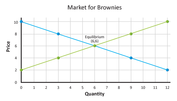
- Ask students to draw a supply curve on the same graph as the demand graph they drew earlier in step 14. Point out the intersection of the drawn supply and demand curves. Ask students what this represents. [Answers will vary. Some students may realize that this is the point at which the quantity supplied equals the quantity demanded.] Show Episode 3: Equilibrium from the Federal Reserve Bank of St. Louis’ Economic Low Down Video Series found at https://www.stlouisfed.org/education/economic-lowdown-video-series/episode-3-equilibrium. Stop the video at 3:15.Discuss:
- Is it supply or demand that determines price? [They both do.]
- What is the point where the supply curve and demand curve intersect called? [Market equilibrium.]
- What does equilibrium mean? [Balance, stability.]
- What does this point represent? [It represents the market clearing or equilibrium price. The price at which the quantity supplied equals the quantity demanded.]
- What is equilibrium quantity? [The quantity supplied and quantity demanded at the equilibrium or market clearing price.]

- Ask students to look at a price of $4 on the graph. Discuss the following:
- What is the quantity supplied at this price? [3]
- What is the quantity demanded at this price? [9]
Explain that typically as the price of a good or service rises (or falls), the quantity of that good or service producers are willing to produce and sell increases (or decreases).
Ask students to look at the price of $8 on the graph. Discuss the following:
- What is the quantity supplied at this price? [9]
- What is the quantity demanded at this price? [3]
Explain that when the quantity supplied is greater than the quantity demanded, there is a surplus. Ask students what they think will happen that will move the market toward equilibrium; that is, eliminate the surplus. (To sell more of the product, producers will reduce the price. At a lower price, consumers will be willing and able to buy more. This process will continue until the market clears—reaches equilibrium.)
- Tell students they are going to use what they have learned about supply and demand to mathematically confirm the equilibrium price and quantity.
- Review and define linear functions. [Linear functions are those whose graph is a straight line.]
- Review and define a system of equations. [A system of linear equations is a collection of linear functions involving the same set of variables, and in our case today two lines that cross each other.]
- Review and define slope. [The slope of a line is the number that describes both the direction and the steepness of the line, most commonly referred to as rise over run.]
- Review how to compute equations for a linear function using data from a function table.
- Use two points from the table to find the slope using the formula

- Use the slope and one of the ordered pairs from the table in the formula

- Solve for

- Once you have the slope and b, which represents the y intercept, you enter the slope and the intercept into the function for the line.
- Use two points from the table to find the slope using the formula
- Distribute a copy of Activity 2 to each student. Explain that they are to utilize Activity 2 and work along with you as you solve the problem. Guide students through the process of using the slope intercept form and the substitution method for systems of equations to confirm equilibrium. First graph the supply and demand curves, then find the equation of the lines. Review answers using Activity 2 Answer Key.
- Distribute a copy of Activity 3 to each student. Give students time to work through the problem in class. Review answers using Activity 3 Answer Key.
- Discuss the following:
- What do economists mean by supply? [The amount of a good or service that producers are willing and able to offer for sale at each possible price during a given period of time.]
- How does this differ from the way the term supply might be used by a friend? [Answers will vary but might include the amount of something an individual has.]
- What do economists mean by demand? [The quantity of a good or service that buyers are willing and able to buy at all possible prices during a period of time.]
- How does this differ from the way a friend might use the term demand? [Answers will vary but might include the amount of something an individual wants.]
- Describe the relationship between quantity supplied and price. [As the price of a good or service rises (or falls), the quantity of that good or service that producers are willing and able to supply during some time period rises (or falls).]
- What is the law of demand? [As the price of a good or service rises (or falls), the quantity of that good or service that people are willing and able to buy during a certain period of time falls (or rises).]
- What is meant by market equilibrium? [The intersection of the supply and demand curves, where they cross; where the quantity supplied equals the quantity demanded. This is also known as the market clearing price and quantity.]
- How can we mathematically confirm the equilibrium point? [Find the equations of the lines, solve for x and y using a system of equations or by graphing the equations and finding their intersection. X=equilibrium quantity, Y=equilibrium price.]
Assessment
- Which statement best describes the relationship between price and quantity supplied?
- As the price of a good increases, the quantity supplied decreases.
- [As the price of a good increases, the quantity supplied increases.]
- As the price of a good decreases, the quantity supplied increases.
- As the price of the good decreases, the quantity supplied remains unchanged.
- What is the formula for the equation of a line?

- b = mx -y
- [y = mx + b]

- Given the following two equations, find where they intersect (equilibrium point): d(x) = -.25x +480 and s(x) = .95x
- Quantity = 380 and Price = 400
- [Quantity = 400 and Price = 380]
- Quantity = 200 and Price = 380
- Quantity = 380 and Price = 200
- Distribute a copy of Activity 4 to each student. Instruct students to use the data to graph the supply and demand curves, find the equations of the lines, and use the system of equations to confirm the equilibrium point. Grade student work using Activity 4 Answer Key.
| Price (y axis) |
Quantity demanded (x axis) |
Price (y axis) |
Quantity demanded (x axis) |
| 14 | 60 | 6 | 60 |
| 8 | 120 | 12 | 120 |
| 2 | 180 | 18 | 180 |